哈喽,大家好~
咱们今天聊聊XGBoost 和随机森林,关于在提升树与投票机制方面的对比。
XGBoost 和随机森林(Random Forest)是两种非常流行的集成学习方法。它们都属于树模型的集成方法,但核心机制不同:
随机森林属于Bagging(Bootstrap Aggregating)的一种,通过并行训练多个决策树,然后通过投票(分类)或平均(回归)来获得最终预测。
XGBoost 是 Boosting 的一种,通过串行训练多个弱学习器(一般是 CART 树),每一轮优化之前模型的残差,采用加法模型与梯度下降思想。
下面,和大家好好细致的聊一下~
模型结构对比
1. 随机森林结构
随机森林训练过程:
对训练集 ,进行有放回采样(Bootstrap),得到多个子数据集 ; 对每个子数据集训练一棵决策树 ; 最终模型是这些树的集成:
特征选择机制:每棵树在分裂节点时随机选择部分特征,增强多样性。
2. XGBoost结构
XGBoost 使用加法模型叠加多个弱学习器(CART 树):
其中:
:所有可用 CART 树的集合; :第 棵树输出的预测值; 每一轮都试图最小化损失函数:
其中 是正则化项,控制模型复杂度,例如:
:树的叶节点数量; :第 个叶节点的得分; :正则化超参数。
训练方式对比
随机森林的并行性与稳定性
各棵树独立训练,可并行处理; 对噪声和过拟合具有鲁棒性(因为投票机制); 不使用残差,不考虑树之间的关系。
XGBoost 的串行优化与残差学习
每棵树的训练依赖于前一棵树的输出; 核心是使用二阶泰勒展开对损失函数近似,使用梯度提升:
损失函数近似公式:
假设当前是第 轮,前 棵树已经得到预测值 ,第 棵树的目标是最小化:
其中:
; ;
最终转化为对树结构的结构评分函数的优化:
其中:
, ; :第 个叶节点中的样本集合。
预测机制对比
随机森林:投票机制:
每棵树独立预测,分类中使用多数投票,回归中使用平均值; 偏差较大但方差较小(多棵树可以降低方差); 对异常值不敏感。
XGBoost:加法模型:
每棵树预测值作为“增量”,不断修正残差; 偏差较小但方差可能大; 更容易拟合复杂结构,风险是可能过拟合(但 XGBoost 有正则项控制)。
一个案例
这里,我构造一个非线性、非对称分布的二维数据集,使得模型必须建模非线性边界才能获得高性能。
样本数:2000 特征维度:2(便于可视化) 类别:2(分类问题)
我们通过 make_moons 加噪声模拟真实复杂边界场景。
import numpy as np
import matplotlib.pyplot as plt
from sklearn.datasets import make_moons
from sklearn.model_selection import train_test_split
from sklearn.ensemble import RandomForestClassifier
from xgboost import XGBClassifier
from sklearn.metrics import (
    accuracy_score, roc_auc_score, confusion_matrix, roc_curve, classification_report
)
import seaborn as sns
import matplotlib.gridspec as gridspec

# 1. 数据准备
X, y = make_moons(n_samples=2000, noise=0.3, random_state=42)
X_train, X_test, y_train, y_test = train_test_split(X, y, test_size=0.3, random_state=42)

# 2. 模型训练
rf = RandomForestClassifier(n_estimators=100, max_depth=5, random_state=42)
xgb = XGBClassifier(use_label_encoder=False, eval_metric='logloss', learning_rate=0.1, n_estimators=100, max_depth=5, random_state=42)

rf.fit(X_train, y_train)
xgb.fit(X_train, y_train)

# 3. 预测
rf_preds = rf.predict(X_test)
xgb_preds = xgb.predict(X_test)

rf_probs = rf.predict_proba(X_test)[:, 1]
xgb_probs = xgb.predict_proba(X_test)[:, 1]

# 4. 可视化准备
fig = plt.figure(figsize=(16, 12))
gs = gridspec.GridSpec(2, 2)

# 图1:决策边界对比
def plot_decision_boundary(ax, model, title):
    h = .02
    x_min, x_max = X[:, 0].min() - .5, X[:, 0].max() + .5
    y_min, y_max = X[:, 1].min() - .5, X[:, 1].max() + .5
    xx, yy = np.meshgrid(np.arange(x_min, x_max, h),
                         np.arange(y_min, y_max, h))
    Z = model.predict(np.c_[xx.ravel(), yy.ravel()])
    Z = Z.reshape(xx.shape)
    cmap_bg = plt.cm.coolwarm
    ax.contourf(xx, yy, Z, cmap=cmap_bg, alpha=0.6)
    scatter = ax.scatter(X_test[:, 0], X_test[:, 1], c=y_test, cmap=cmap_bg, edgecolor='k', s=20)
    ax.set_title(title)
    ax.set_xlabel("Feature 1")
    ax.set_ylabel("Feature 2")

ax1 = plt.subplot(gs[0, 0])
plot_decision_boundary(ax1, rf, "Random Forest 决策边界")

ax2 = plt.subplot(gs[0, 1])
plot_decision_boundary(ax2, xgb, "XGBoost 决策边界")

# 图2:ROC 曲线
fpr_rf, tpr_rf, _ = roc_curve(y_test, rf_probs)
fpr_xgb, tpr_xgb, _ = roc_curve(y_test, xgb_probs)

ax3 = plt.subplot(gs[1, 0])
ax3.plot(fpr_rf, tpr_rf, label="Random Forest", color='blue')
ax3.plot(fpr_xgb, tpr_xgb, label="XGBoost", color='darkorange')
ax3.plot([0, 1], [0, 1], 'k--', alpha=0.7)
ax3.set_title("ROC 曲线对比")
ax3.set_xlabel("False Positive Rate")
ax3.set_ylabel("True Positive Rate")
ax3.legend(loc="lower right")
ax3.grid(True)

# 图3:混淆矩阵
cm_rf = confusion_matrix(y_test, rf_preds)
cm_xgb = confusion_matrix(y_test, xgb_preds)

ax4 = plt.subplot(gs[1, 1])
sns.heatmap(cm_rf, annot=True, fmt='d', cmap='Blues', cbar=False, ax=ax4, xticklabels=[0, 1], yticklabels=[0, 1])
ax4.set_title("随机森林混淆矩阵")
ax4.set_xlabel("Predicted")
ax4.set_ylabel("Actual")

plt.tight_layout()
plt.show()
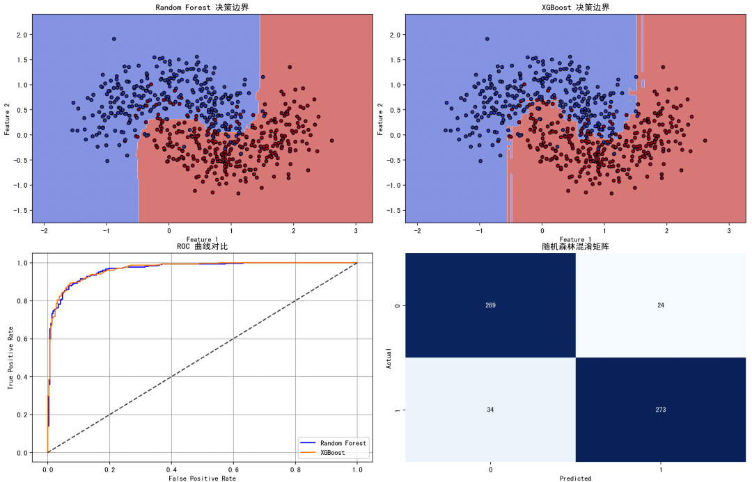
图1:决策边界对比(左上 & 右上)
随机森林:边界较为“阶梯状”,反映了其以多数投票划分空间; XGBoost:边界更光滑,能更好拟合数据的“月牙形”结构,显著提升边界精度。
图2:ROC 曲线对比(左下)
XGBoost 曲线下方面积更大(AUC 更高),意味着它能更好地区分两个类别。
图3:混淆矩阵(右下)
可清楚看出各模型在分类正确与错误的数量; XGBoost 错误率更低,表明其分类精度更高。
随机森林适用场景:
快速构建基线模型; 数据量较大但特征重要性分析为主; 不易过拟合,适用于高方差场景; 用户对模型可解释性有一定要求。
XGBoost适用场景:
需要最高预测精度(如 Kaggle 比赛、金融风控、CTR 预测等); 数据非线性边界复杂; 可以接受较长训练时间; 熟练掌握调参(可结合 GridSearch、Optuna 等)。
随机森林和XGBoost虽然都是树模型的集成策略,但在训练方式、误差优化方式与模型结构上有本质不同。在应用中,建议根据数据规模、训练时间要求、解释性需求以及业务精度要求选择对应算法。
最后