哈喽,大家好~
咱们今天聊聊随机森林和XGBoost性能评测。
随机森林和XGBoost是两种广泛使用的集成学习方法,在机器学习任务中常用于分类和回归问题。
两者的核心思想虽然都是通过集成多个决策树来提高模型性能,但其训练方式、模型结构、泛化能力和运行效率有本质区别。
一、算法原理
随机森林
核心思想:Bagging(Bootstrap Aggregating)
流程:
从训练集中有放回地随机抽样生成多个子训练集。 每个子训练集训练一棵决策树。 每棵树训练时节点分裂只考虑部分特征(特征子集)。 最终预测结果通过多数投票(分类)或平均(回归)合并。
预测公式:
对于分类任务:
对于回归任务:
其中, 是第 棵树的预测结果, 为树的总数。
XGBoost
核心思想:Boosting + 梯度优化
流程:
迭代地训练树模型,每次拟合前一轮的残差(梯度)。 使用二阶泰勒展开进行目标函数优化。 引入正则项控制模型复杂度(防止过拟合)。
目标函数(带正则项):
其中,
是损失函数(如平方误差或对数损失); 是第 棵树; 为正则项,控制树的复杂度; 是叶子数, 是第 个叶子的分数。
使用二阶近似展开优化:
其中,
为一阶导数; 为二阶导数。
二、性能对比指标
我们从以下几个方面进行评估:
准确率(Accuracy)/ 均方误差(MSE)
分类任务
通常评估准确率(Accuracy)、F1-score、AUC 等。
回归任务
常用指标为均方误差(MSE):
对比:
XGBoost 通常优于随机森林,尤其在复杂非线性关系下。 随机森林更稳定,在小样本或高噪声下表现更稳健。
偏差-方差分解
随机森林
方差降低明显(通过Bagging平均多个弱分类器)。 偏差不变或略高。
XGBoost
偏差降低(通过迭代修正残差)。 方差可能上升(模型更复杂,需正则项调控)。
完整案例
好的,下面是一个完整的案例,内容包含:
虚拟数据生成 模型训练:随机森林(Random Forest) vs XGBoost 性能评估 数据可视化** 详细分析与总结:各自的优势、适用场景
第一步:导入库与数据生成
import numpy as np
import pandas as pd
import matplotlib.pyplot as plt
import seaborn as sns
from sklearn.datasets import make_classification
from sklearn.ensemble import RandomForestClassifier
from xgboost import XGBClassifier
from sklearn.model_selection import train_test_split, cross_val_score
from sklearn.metrics import classification_report, confusion_matrix, roc_auc_score, roc_curve, accuracy_score
import warnings
warnings.filterwarnings('ignore')

# 设置风格
sns.set(style="whitegrid")
plt.rcParams['font.family'] = 'Arial'
生成虚拟数据集
# 生成一个包含多特征的二分类数据集
X, y = make_classification(n_samples=1000, n_features=20,
                           n_informative=10, n_redundant=5,
                           n_clusters_per_class=2, random_state=42)

# 转为DataFrame格式
df = pd.DataFrame(X, columns=[f'Feature_{i}' for i in range(1, 21)])
df['Target'] = y

# 数据划分为训练集和测试集
X_train, X_test, y_train, y_test = train_test_split(df.drop('Target', axis=1),
                                                    df['Target'],
                                                    test_size=0.3,
                                                    random_state=42)
第二步:模型训练与性能比较
# 初始化模型
rf_model = RandomForestClassifier(n_estimators=100, random_state=42)
xgb_model = XGBClassifier(use_label_encoder=False, eval_metric='logloss', random_state=42)

# 模型训练
rf_model.fit(X_train, y_train)
xgb_model.fit(X_train, y_train)

# 预测
rf_pred = rf_model.predict(X_test)
xgb_pred = xgb_model.predict(X_test)

# 概率预测(用于ROC绘制)
rf_prob = rf_model.predict_proba(X_test)[:, 1]
xgb_prob = xgb_model.predict_proba(X_test)[:, 1]
第三步:性能评估指标
# 输出准确率与AUC
print("Random Forest Accuracy:", accuracy_score(y_test, rf_pred))
print("XGBoost Accuracy:", accuracy_score(y_test, xgb_pred))

print("Random Forest AUC:", roc_auc_score(y_test, rf_prob))
print("XGBoost AUC:", roc_auc_score(y_test, xgb_prob))
第四步:可视化对比分析
图1:混淆矩阵对比
fig, axes = plt.subplots(1, 2, figsize=(14, 6))
sns.heatmap(confusion_matrix(y_test, rf_pred), annot=True, fmt='d', ax=axes[0], cmap='Blues')
axes[0].set_title("Random Forest Confusion Matrix")
axes[0].set_xlabel("Predicted")
axes[0].set_ylabel("Actual")

sns.heatmap(confusion_matrix(y_test, xgb_pred), annot=True, fmt='d', ax=axes[1], cmap='Oranges')
axes[1].set_title("XGBoost Confusion Matrix")
axes[1].set_xlabel("Predicted")
axes[1].set_ylabel("Actual")

plt.tight_layout()
plt.show()
可视化各模型预测分类的精度,越对角分布越好

图2:ROC曲线对比
fpr_rf, tpr_rf, _ = roc_curve(y_test, rf_prob)
fpr_xgb, tpr_xgb, _ = roc_curve(y_test, xgb_prob)

plt.figure(figsize=(10, 6))
plt.plot(fpr_rf, tpr_rf, label='Random Forest', color='blue')
plt.plot(fpr_xgb, tpr_xgb, label='XGBoost', color='orange')
plt.plot([0, 1], [0, 1], 'k--')
plt.xlabel("False Positive Rate")
plt.ylabel("True Positive Rate")
plt.title("ROC Curve Comparison")
plt.legend()
plt.grid(True)
plt.show()
展示二分类模型整体性能,曲线越贴近左上角性能越佳。

图3:特征重要性对比
rf_importance = rf_model.feature_importances_
xgb_importance = xgb_model.feature_importances_

feat_df = pd.DataFrame({
    'Feature': X_train.columns,
    'Random Forest': rf_importance,
    'XGBoost': xgb_importance
}).set_index('Feature')

feat_df.sort_values("Random Forest", ascending=False).head(10).plot.bar(figsize=(12, 6), colormap='viridis')
plt.title("Top 10 Feature Importance Comparison")
plt.ylabel("Importance Score")
plt.xlabel("Feature")
plt.grid(True)
plt.tight_layout()
plt.show()
了解模型依赖哪些特征,有助于做特征工程。

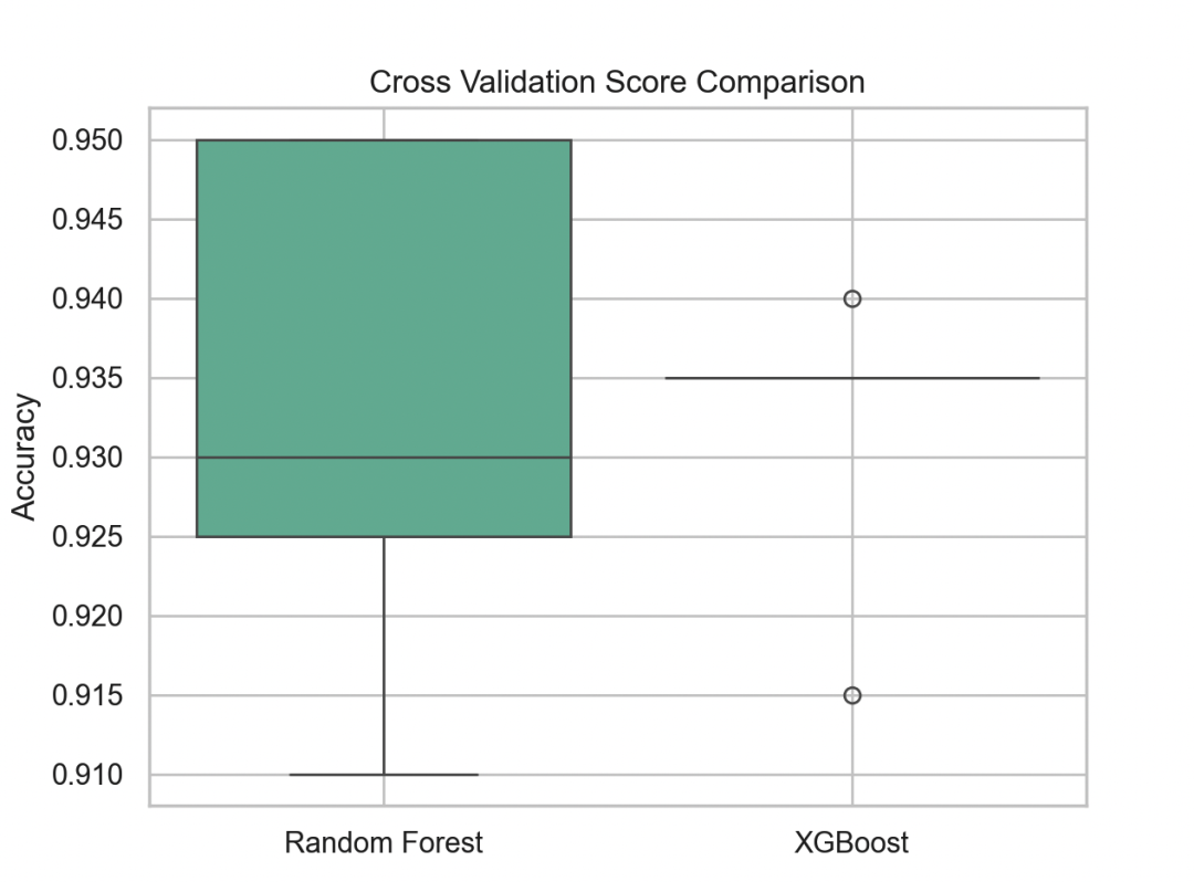
图4:交叉验证得分箱线图
rf_scores = cross_val_score(rf_model, X, y, cv=5)
xgb_scores = cross_val_score(xgb_model, X, y, cv=5)

score_df = pd.DataFrame({
    'Random Forest': rf_scores,
    'XGBoost': xgb_scores
})

sns.boxplot(data=score_df, palette='Set2')
plt.title("Cross Validation Score Comparison")
plt.ylabel("Accuracy")
plt.grid(True)
plt.show()
通过交叉验证展示模型稳定性,箱体越紧说明方差越小。
最后