哈喽,大家好~
今儿和大家一起来看看随机森林 vs XGBoost,提升树与投票机制的对比,还有哪些是我们要着重学习的~
随机森林
随机森林是一种 Bagging(Bootstrap Aggregating)+ 决策树 的方法。
核心思想是:
从训练集 中 有放回地抽样 出 个子集 。 在每个子集上训练一棵决策树 ,通常是 CART回归或分类树。 对所有树的预测结果进行 投票(分类)或平均(回归) 得到最终预测:
假设回归问题中单棵树误差为 ,并且树之间的相关系数为 ,随机森林平均后的方差为:
当树之间不相关 (),方差完全按 缩小。 树之间高度相关时,方差降低有限。
核心特点:
多棵树 并行训练,互相独立。 投票/平均是 等权重。 重点是 降低方差,偏差通常较高(每棵树深度大时偏差低,但单棵树容易过拟合)。
XGBoost
XGBoost 属于 Boosting,核心是 逐步拟合残差的加法模型:
是第 棵树。 每棵树的目标是 拟合当前模型残差:
这里 是损失函数(如均方误差、对数损失等)。
XGBoost 的目标函数是带正则化的损失:
其中,正则化项
= 树叶节点数 = 叶节点权重 = 正则化系数
通过二阶泰勒展开近似优化:
其中:
树的最优叶子权重为:
最终树的分裂增益:
核心特点:
树 顺序训练,后一棵树拟合前面树的残差。 每棵树 权重不同,由梯度方向决定。 重点是 降低偏差,也兼顾方差(正则化)。
投票机制 vs 提升树机制
简单理解:
随机森林像“民主投票”,每棵树独立表决,平均结果。 XGBoost像“有策略的接力赛”,每一棒(树)都修正前面棒的不足(残差)。
完整案例
这里的案例,给出 3 个目标:
对比两种算法在同一数据集上的拟合效果和预测能力。 可视化分析模型差异,包括:
模型拟合曲线 残差分布 特征重要性 局部预测差异
这里使用一个非线性回归数据集:
代码:
import numpy as np
import pandas as pd
import matplotlib.pyplot as plt
import seaborn as sns

from sklearn.model_selection import train_test_split
from sklearn.ensemble import RandomForestRegressor
from xgboost import XGBRegressor
from sklearn.metrics import mean_squared_error


# 生成虚拟数据集
np.random.seed(42)
N = 500
x1 = np.random.uniform(-5, 5, N)
x2 = np.random.uniform(-5, 5, N)
epsilon = np.random.normal(0, 0.5, N)

y = 5 * np.sin(x1) + 3 * np.log(np.abs(x2) + 1) + epsilon

# 构建DataFrame
df = pd.DataFrame({'x1': x1, 'x2': x2, 'y': y})

# 划分训练集与测试集
X = df[['x1', 'x2']]
y = df['y']
X_train, X_test, y_train, y_test = train_test_split(X, y, test_size=0.2, random_state=42)
模型训练与预测
随机森林:
# 随机森林
rf_model = RandomForestRegressor(n_estimators=200, max_depth=6, random_state=42)
rf_model.fit(X_train, y_train)
y_pred_rf = rf_model.predict(X_test)
mse_rf = mean_squared_error(y_test, y_pred_rf)
print("Random Forest MSE:", mse_rf)
XGBoost:
# XGBoost
xgb_model = XGBRegressor(n_estimators=200, max_depth=6, learning_rate=0.1, random_state=42)
xgb_model.fit(X_train, y_train)
y_pred_xgb = xgb_model.predict(X_test)
mse_xgb = mean_squared_error(y_test, y_pred_xgb)
print("XGBoost MSE:", mse_xgb)
数据分析可视化
# 创建网格用于曲面图
x1_grid = np.linspace(-5, 5, 50)
x2_grid = np.linspace(-5, 5, 50)
x1_mesh, x2_mesh = np.meshgrid(x1_grid, x2_grid)
grid = pd.DataFrame({'x1': x1_mesh.ravel(), 'x2': x2_mesh.ravel()})

# 预测曲面
y_grid_rf = rf_model.predict(grid).reshape(50, 50)
y_grid_xgb = xgb_model.predict(grid).reshape(50, 50)

# 绘制四个子图
fig, axes = plt.subplots(2, 2, figsize=(20, 16))

# 图1:真实 vs 预测
axes[0,0].scatter(y_test, y_pred_rf, color='tomato', alpha=0.6, label='RF')
axes[0,0].scatter(y_test, y_pred_xgb, color='dodgerblue', alpha=0.6, label='XGB')
axes[0,0].plot([y.min(), y.max()], [y.min(), y.max()], 'k--', lw=2)
axes[0,0].set_xlabel("True y")
axes[0,0].set_ylabel("Predicted y")
axes[0,0].set_title("True vs Predicted Values")
axes[0,0].legend()

# 图2:残差分布
res_rf = y_test - y_pred_rf
res_xgb = y_test - y_pred_xgb
sns.histplot(res_rf, bins=20, color='tomato', alpha=0.6, label='RF Residual', ax=axes[0,1])
sns.histplot(res_xgb, bins=20, color='dodgerblue', alpha=0.6, label='XGB Residual', ax=axes[0,1])
axes[0,1].set_title("Residual Distribution")
axes[0,1].legend()

# 图3:特征重要性
feat_imp_rf = pd.Series(rf_model.feature_importances_, index=X.columns)
feat_imp_xgb = pd.Series(xgb_model.feature_importances_, index=X.columns)
feat_imp_rf.plot(kind='bar', color='tomato', alpha=0.7, ax=axes[1,0], label='RF')
feat_imp_xgb.plot(kind='bar', color='dodgerblue', alpha=0.7, ax=axes[1,0], label='XGB')
axes[1,0].set_title("Feature Importance")
axes[1,0].legend()

# 图4:预测曲面
cont1 = axes[1,1].contourf(x1_mesh, x2_mesh, y_grid_rf, cmap='Reds', alpha=0.6)
cont2 = axes[1,1].contourf(x1_mesh, x2_mesh, y_grid_xgb, cmap='Blues', alpha=0.4)
axes[1,1].scatter(X_test['x1'], X_test['x2'], c=y_test, edgecolor='k', cmap='viridis', s=60)
axes[1,1].set_title("Prediction Surface: RF(Red) vs XGB(Blue)")

plt.tight_layout()
plt.show()
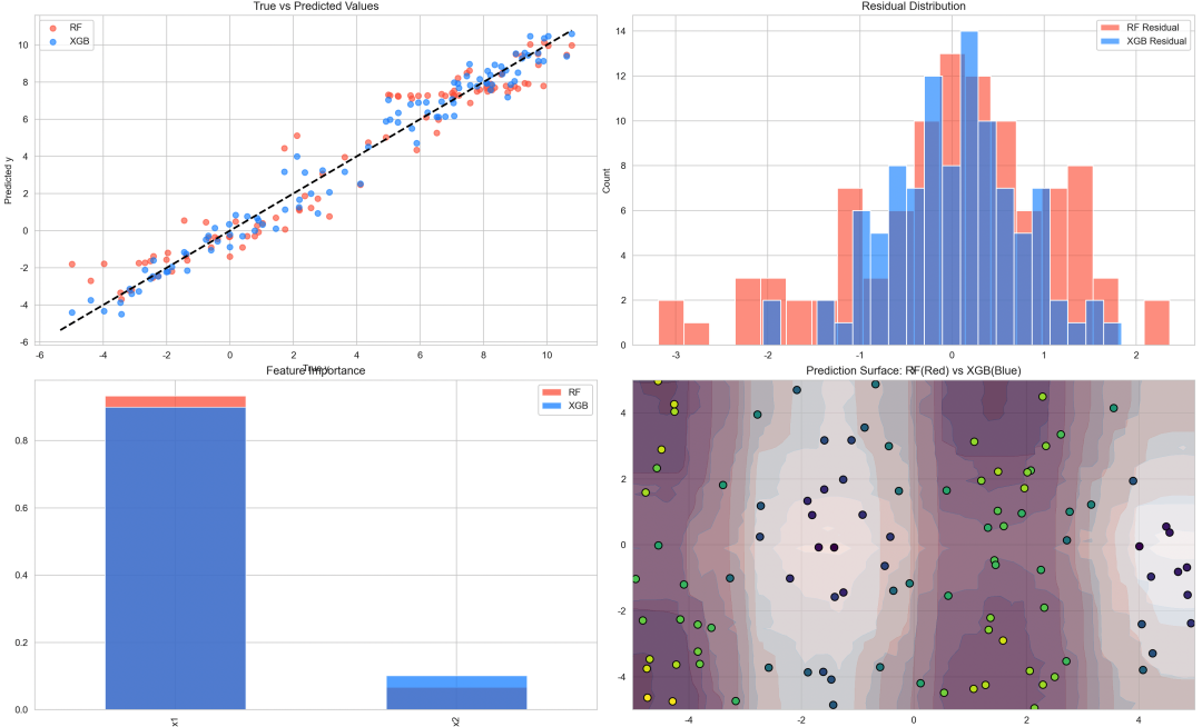
图 1(真实值 vs 预测值)
RF 和 XGB 都能拟合整体趋势。 XGB 曲线更贴近对角线,说明 Boosting 更善于捕捉非线性复杂关系。
图 2(残差分布)
RF 残差分布稍宽,说明存在部分系统偏差。 XGB 残差分布更集中,说明偏差降低效果好。
图 3(特征重要性)
两者都认定 x1对目标影响更大。XGB 更强调 x1,说明 Boosting 对主要特征敏感度更高。
图 4(预测曲面)
RF 曲面较平滑,部分细节被平均。 XGB 曲面更精细,非线性拟合效果更明显。 红色(RF)与蓝色(XGB)叠加可以直观看出差异。
总体来讲,随机森林通过投票/平均降低方差,适合快速、稳定的建模场景。
XGBoost通过提升树顺序拟合残差降低偏差,适合复杂非线性数据。
最后

